
When requests arrive together, they can have to wait before a query even starts because no database connection is available. Increasing the connection pool—the set of database connections kept for reuse—looks like a way to reduce that wait.
But reducing connection wait is not the only question. Will the time until query results arrive get shorter too? To find out, we used the same Postgres database with 5, 20, and 100 connections and measured the time before and after borrowing a connection separately.
In the experiment, sending 10 queries together with 5 connections produced a mean wait of 22.1ms to borrow a connection. With 20 connections, that wait was almost zero. Yet the mean time for the whole operation, including returning the connection, grew from 72.3ms to 95.7ms.
Under these conditions, less connection wait did not by itself mean the whole operation had improved. Below, we examine which intervals grew and explain what to record before and after changing connection counts in your own application.
We sent a fixed number of requests to a small database limited to 0.5 CPU core. This does not establish maximum capacity or an optimal connection count for every environment.
Measure before and after borrowing a connection separately
A task running a search or other query borrows a connection before running a query and returns it afterward. If none is available, it waits to borrow one. The official asyncpg documentation shows this acquire-and-release pattern.
We used Python's asyncpg and pool limits of 5, 20, and 100. In every condition, we established that full number of connections in advance. The measurement does not include opening a new connection for each request.
The database's max_connections stayed at 110 in every condition. That is the maximum number of concurrent connections Postgres accepts, a different setting from the application pool limit varied here. See the PostgreSQL connection settings.
to task startScheduling delay
from the poolAcquisition wait
and receive resultsQuery round trip
to the poolRelease
We defined overall time as the interval from the scheduled send time until connection release completed. We also recorded when a connection was acquired and when the SQL result arrived. Release includes asyncpg's standard connection reset.
“Query round trip” is elapsed time measured on the client. It is not pure SQL execution time inside the database: it includes database work and waiting, as well as client-side handling of the result.
Acquisition wait almost disappeared, but the overall mean grew
We list the mean times of the four intervals for batches of 10. The overall time and each interval are averages over the same requests.
| Mean time with bursty arrivals | 5 connections | 20 connections | 100 connections |
|---|---|---|---|
| Scheduled send to task start | 1.7ms | 2.0ms | 2.2ms |
| Pool acquisition wait | 22.11ms | 0.03ms | 0.03ms |
| Query round trip | 38.4ms | 79.9ms | 80.3ms |
| Pool release | 10.1ms | 13.8ms | 13.8ms |
| Overall | 72.3ms | 95.7ms | 96.4ms |
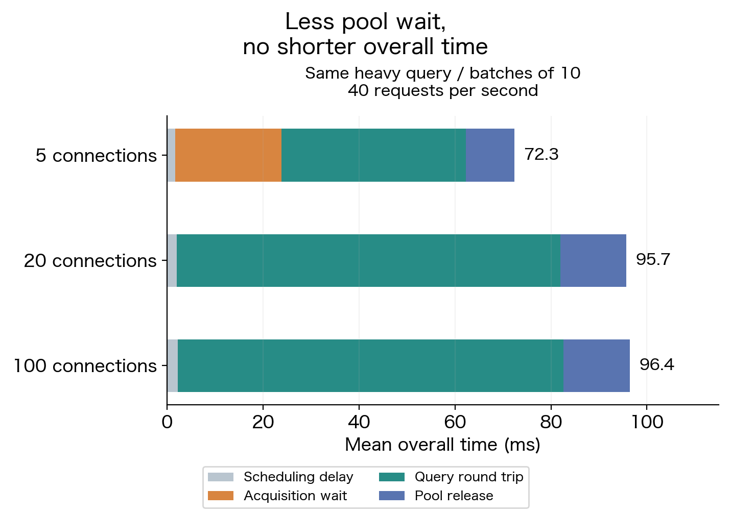
With 5 connections, some of the 10 simultaneous requests wait before borrowing a connection. With 20 or 100, all 10 can borrow one, and that wait almost disappears. Meanwhile, the mean query round trip grows from about 38ms to 80ms. Including release, the overall mean grows as well.
The measurement shows that less acquisition wait and more time after acquisition were observed together. It does not mean the 22ms saved simply moved elsewhere. Nor can these records separate how many milliseconds were spent waiting in each part of the query round trip.
More connections allow more work to be sent to the database. In this experiment, however, we did not increase the total CPU available to it. The number of requests allowed to proceed and the amount of computation that can actually progress are separate questions.
Send three workloads to the same database
We prepared 20,000 rows, about 3.8MiB including the table and index. The light query fetches one row by primary key. The heavy query computes MD5 hashes of strings across 2,000 rows and aggregates the result. “Heavy” describes a comparison workload involving computation, not a reproduction of a production query.
-- Light query
SELECT balance FROM pool_lab WHERE id = $1;

-- Heavy query
SELECT sum(length(md5(payload || id::text)))
FROM pool_lab
WHERE id BETWEEN $1 AND $1 + 1999;
We used the following three arrival patterns, scheduling requests in advance rather than waiting for each response before sending the next.
| Condition | Scheduled arrivals | Measurements per pool setting |
|---|---|---|
| Light query, uniform arrivals | 1 every 5ms, 200/sec | 7,200 |
| Heavy query, uniform arrivals | 1 every 25ms, 40/sec | 1,440 |
| Heavy query, bursty arrivals | 10 every 250ms, 40/sec | 1,440 |
The two heavy-query conditions use the same SQL and mean request rate. What changes is whether requests arrive in short bursts. The light and heavy queries have different arrival rates, so we do not use them to calculate a performance multiplier between queries.
The entire database was limited to 0.5 CPU core, with a separate 0.5-core limit for the load generator. The quota period was 10ms. After executing the SQL on each connection in advance, we warmed up for 2 seconds and measured three 12-second runs per condition. Pool order was varied across the 27 runs, and all 30,240 requests completed.
Compare slower responses and bursts of arrivals too
Averages can make it difficult to see delays affecting some responses. We therefore also compare response times at the slower end. For example, with 100 observations sorted from fastest to slowest, this is the time of the 99th response. The table below pools all three runs of each condition. This is a different measure from the means above.
| Arrival condition | 5 connections | 20 connections | 100 connections |
|---|---|---|---|
| Light, uniform 200/sec | 1.90ms | 1.88ms | 1.94ms |
| Heavy, uniform 40/sec | 11.22ms | 14.69ms | 13.63ms |
| Heavy, batches of 10 at 40/sec | 125.98ms | 133.19ms | 132.09ms |
For the light query, the response time at the slower end stayed around 1.9ms as the connection count changed. Uniform arrivals of the heavy query also showed no pattern of shorter response times at the slower end with more connections.
The much larger difference came from how we sent the same 40 requests per second. With batches of 10, response time at the slower end was about 126–133ms.
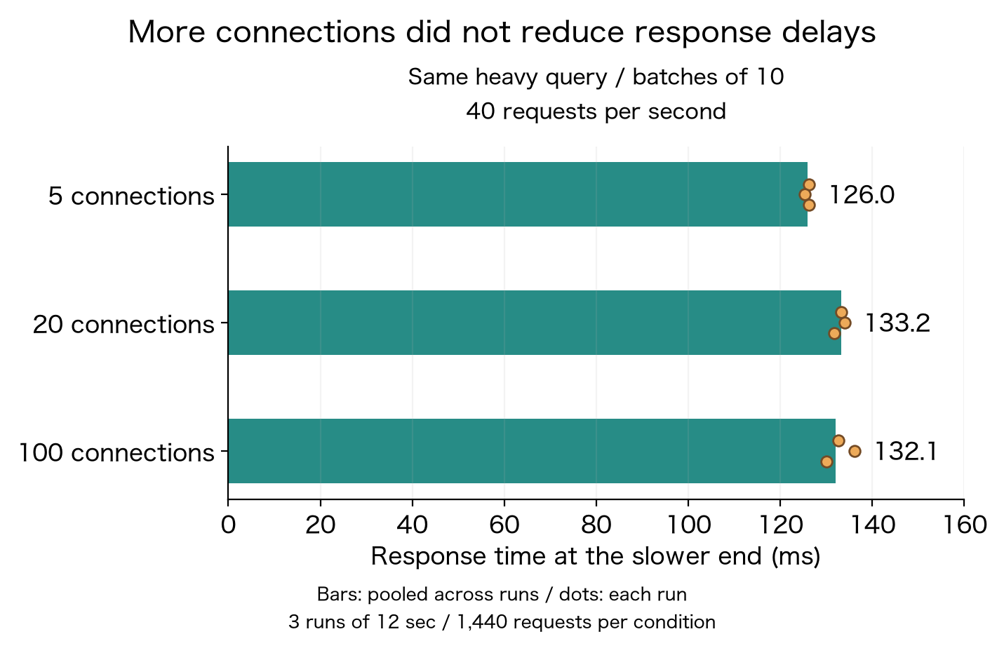
Values calculated the same way for individual runs also varied: 125.3–126.3ms with 5 connections, 131.8–134.0ms with 20, and 130.0–136.2ms with 100 under bursty arrivals. These are the minimum and maximum across three runs, not confidence intervals. Rather than treating small differences as a general ranking, we read this as no improvement from increasing connections under these conditions.
Completed throughput was about 200 requests/sec for the light query and 40 requests/sec for either heavy-query pattern. This means the configured arrival rate was handled. We did not raise that rate to find a limit, so it does not mean every pool has a maximum capacity of 40 requests/sec.
Short bursts can hit a quota despite low average CPU usage
Linux cgroups limited all database processes together to 5ms of CPU time per 10ms period. Running multiple tasks concurrently does not increase the group's total budget. The official Linux kernel documentation explains these settings and counters.
With bursty arrivals, mean database CPU usage was 0.247 core with 5 connections, 0.260 with 20, and 0.265 with 100. That is about 49–53% of the configured 0.5-core limit.
Throttling still occurred. The ratio of throttled periods (nr_throttled) to periods recorded in cpu.stat (nr_periods) was about 84–85% with bursty arrivals, calculated from the counter increases during measurement. This is neither a share of total elapsed time nor the percentage of time spent waiting. See also the kernel documentation on statistics. A long-interval average and what happens within a short quota period describe different things.
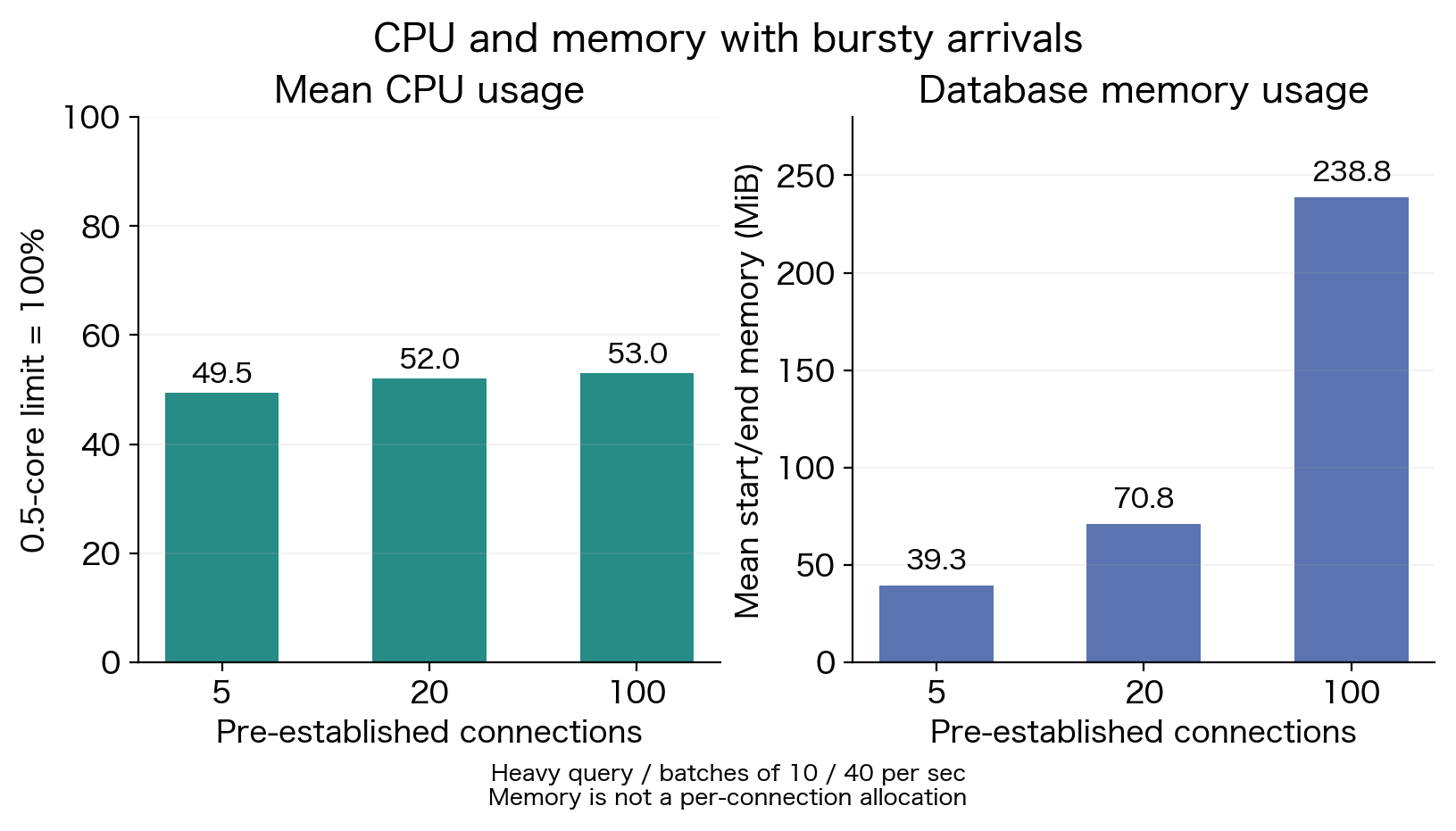
The CPU quota is a clue when investigating time after acquisition. However, we did not run a control without that quota. Throttled-period counts cannot directly reveal an individual request's waiting time. We therefore do not attribute all the latency in this experiment to CPU throttling alone.
Memory also changed. With bursty arrivals, database cgroup usage grew from about 39MiB to 239MiB. We established every connection up to the pool limit beforehand. This does not show that merely configuring a limit of 100 in an application using few actual connections would cause the same growth.
Environment, aggregation, and resumed measurements
The environment was a Raspberry Pi 5, Linux/aarch64, 4 logical CPUs, PostgreSQL 16.13, Python 3.11.2, and asyncpg 0.31.0. Connections used a Unix socket on the same machine, which also ran other work.
Database memory was capped at 768MiB, with shared_buffers=64MiB and work_mem=1MiB. JIT and parallel queries were disabled. This read-only experiment used a small, warmed-up dataset; it cannot establish trends for writes, lock contention, disk I/O, or remote database connections.
We created each pool with min_size=0, acquired connections sequentially until all 5, 20, or 100 were established, executed SQL in advance, and returned them. Idle connection timeouts were disabled, and the actual connection count was verified before measurement.
Overall time includes the delay from a scheduled arrival until the task actually starts. Sorting these start delays and using the same method as in the body gives about 1.3–2.1ms with uniform arrivals and 6.1–7.3ms with bursts. The response time at the slower end is the ceil(count × 0.99)-th sorted value for each condition. CPU usage was the increase in usage_usec divided by observation duration, then aggregated across runs using observation duration as the weight.
Measurements span two blocks separated by a safety stop. After 11 runs, host load exceeded the safety threshold. We recreated the temporary database with the same settings and data for the remaining 16 runs. On resuming, we changed post-measurement connection shutdown to run sequentially. SQL, arrival schedules, resource caps, and warm-up during measurement were unchanged. This was not a strictly continuous experiment, which is another comparison limitation.
An earlier preliminary trial with 100 workers used a different approach after a safety stop and is excluded from this aggregation. We removed the temporary database, services, and files after the experiment and confirmed none remained.
Measurement data
The condition summaries, all 27 runs, 30,240 request measurements, and field and aggregation notes are attached. Internal monitoring records are excluded.
Conclusion: compare connection wait and overall time together
We started by asking whether increasing a pool to reduce database connection wait would also make the whole operation faster. Under these conditions, connection wait almost disappeared, but sending a query and receiving its result took longer, and the overall operation did not get faster.
If you find connection wait in your own application, you can check it in this order.
- Record overall response time and database-call timing before changing settings. For a web application, first record the time until the API or page responds. Around the database call, record four timestamps: immediately before requesting a connection, immediately after obtaining it, immediately after receiving the SQL result, and immediately after returning the connection. Differences between adjacent timestamps give connection wait, query round-trip time, and release time.
- Change only the connection count, record the same measures, and compare them. Keep the SQL, request count, and arrival intervals consistent. Check how the overall response and each interval after acquisition change, as well as connection wait.
- If connection wait falls but the whole operation does not get faster, investigate what follows acquisition before increasing the count again. Check the time from sending SQL to receiving results, database CPU usage and quotas, and connection release. Here, looking only at acquisition wait would have missed the query round trip growing from about 38ms to 80ms.
If more connections also shorten the overall response, that is evidence of improvement for the arrival pattern tested. Check database memory and CPU changes at the same time. Under this experiment's conditions, with every connection established in advance, more connections also meant more memory usage.
The largest batch here was 10 requests. Both 20 and 100 connections let those 10 borrow connections at the same time. These results do not cover 100 simultaneous arrivals or work with long network waits.
This experiment alone cannot tell you how many connections to configure. If you change the setting to reduce connection wait, also check whether the user's overall wait became shorter. Assess improvement after comparing both.
Publish your web app
If you want to run a web app stored on GitHub in a Japan region, KamuiDash lets you deploy it from its repository.